Today we completed the first empirical population of the Θ–Ϟ Transformation Table using the atlas corpus generated by the Cartographer engine.

The goal of this experiment was simple:

Take the dynamical atlases we have already produced across many systems and see whether they could be organized into a small number of transformation geometries.

The result is surprisingly structured.

Across 36 different dynamical systems, spanning neural models, reaction–diffusion systems, ecological models, chaotic maps, and coupled oscillators, each system can be placed into a 4×4 transformation grid defined by two quantities.

The Two Axes

Persistence (Θ)

Persistence measures how strongly a system maintains a stable regime.

It is estimated from atlas features such as:

• basin dominance
• regime concentration
• scale similarity across partitions

High Θ systems maintain large stable regions of behavior.

Instability (Ϟ)

Instability measures how much transition pressure exists in the system.

It is estimated from:

• seam density
• boundary complexity
• regime fragmentation

High Ϟ systems sit near frequent regime transitions.

---

Together these form a transformation coordinate system:

Persistence (Θ)
↑
|
|
|
+--------------------------→ Instability (Ϟ)

Each system becomes a point in this space.

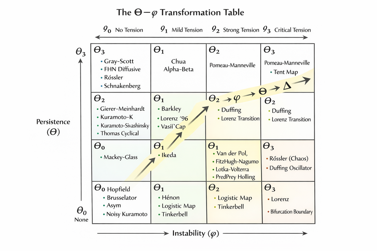
The Transformation Table

Placing the 36 systems into the grid produces the following population pattern.

Θ\Ϟ	0	1	2	3
3	4	1	1	3
2	4	3	1	1
1	1	1	4	3
0	0	4	3	2

Several cells contain four independent systems, suggesting natural transformation families.

Θ₃Ϟ₀ — Stable regime dominated

Systems:

• Gray–Scott
• Schnakenberg
• Rössler
• FitzHugh–Nagumo (diffusive)

These atlases show extremely large attractor basins and minimal regime seams.

Θ₂Ϟ₀ — Stable but structured systems

Systems:

• Gierer–Meinhardt
• Kuramoto
• Kuramoto–Sivashinsky
• Thomas cyclical

These systems maintain dominant regimes but exhibit more internal structure.

Θ₁Ϟ₂ — Oscillatory biological systems

Systems:

• Van der Pol
• FitzHugh–Nagumo
• Lotka–Volterra
• predator–prey (Holling II)

Despite coming from completely different scientific domains, these models occupy the same transformation class.

Θ₀Ϟ₁ — Weak persistence systems

Systems:

• Hopfield
• Brusselator
• asymmetric oscillator
• noisy Kuramoto

These systems exhibit moderate instability but lack strong basin dominance.

Glyph Sequences

Each atlas also produces sequences of glyph operators representing transformation structure.

The canonical transformation sequence is:

`Θ → Ϟ → Я → Ꙩ → Δ

which corresponds to:

persistence → tension → recursion → containment → emergence

The dominant glyph patterns inside table cells are surprisingly consistent.

Cells with moderate persistence and strong instability often show: `

`Θ → Я → Ꙩ → Δ

Cells with higher persistence often show:

Θ → Ϟ → Я → Ꙩ → Δ`

This suggests the glyph layer is capturing structural aspects of the underlying dynamical geometry.

The Diagonal — The Hippasus Path

A particularly interesting feature appears along the diagonal:

Θ₃Ϟ₀ → Θ₂Ϟ₁ → Θ₁Ϟ₂ → Θ₀Ϟ₃

Moving along this path we observe:

• decreasing persistence
• increasing instability
• increasing glyph complexity

This diagonal traces the progression from stable systems toward chaotic transitions.

We have started referring to this trajectory as the Hippasus diagonal, after the mathematician associated with the discovery that certain numerical systems contain internal contradictions that force the emergence of new structures.

What This Suggests

The early evidence indicates that very different equations may share the same transformation geometry.

Neural models, ecological systems, chemical reactions, and chaotic maps can occupy the same transformation cells.

If this continues to hold as the dataset grows, it suggests that:

the geometry of transformation may be more universal than the equations that generate it.

In other words, many systems differ in detail while sharing the same structural transitions.

Next Steps

Three immediate follow-ups are planned.

1. Glyph entropy

Measure the diversity of glyph sequences within each cell.

Low entropy would indicate stable transformation families.

2. Case studies

Trace the full projection for several systems:

equations → atlas → glyph sequence → transformation class

3. Expanding the dataset

Add additional dynamical systems to see whether currently empty cells eventually populate.

Why This Matters

Most dynamical systems research studies individual equations.

The atlas approach instead studies the space of behaviors those equations produce.

The Θ–Ϟ table is an attempt to organize those behaviors into a small number of recurring geometric types.

It is early work.

But today's experiment suggests that such a taxonomy may be possible.

If so, the result could become a kind of periodic table for dynamical transformations.

---

---